Introduction

There are many cases where where a radionuclide decays into a second radionuclide or even long series of concecutive radionuclei. In such cases the disintegration rate of the second radionuclide (we usually refer to this as the "daughter") depend on the decay rate of the first radionuclide (the "mother"). You will find this explained in great detail in your course book and on-line (Google it!).

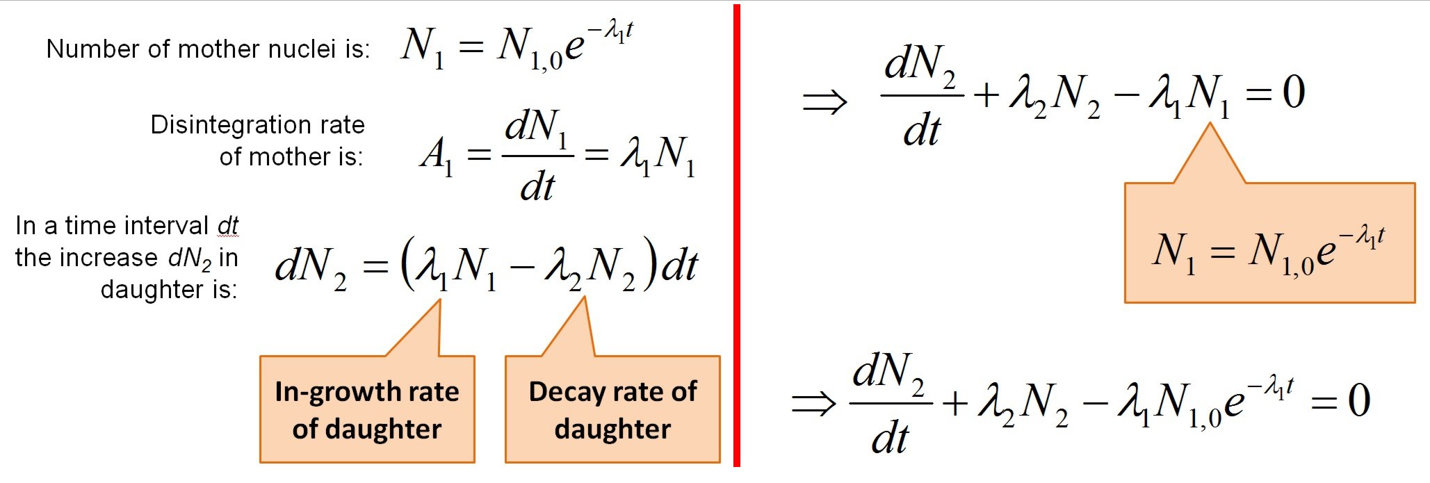
To the right is a brief review of how the differential equation for the rate-change expression for the amount of daughter is derived (click on the picture for a larger version). The parameters have the usaul names, N for the amount (number) of each nuclei, λ is the disintegration constant, and the indexes is 1 for mother and 2 for daughter. The time, t, is the independent variable.

In this exercise you can either use numerical methods to solve this equation or you can use the analytically derived mathematical solution. We suggest that you do both.

Analytical Solution

The analytical solution to the differential equation is:

Here we have introduced the disintegration rate A=λN instead of the amounts of the two nuclei.

How this equation is derrived is explained in basic math courses and has probably also been explained by your NRC teacher. It is not very complicated, but involves a few standard "tricks" and takes some time. We will not explain it here, but you can find it explained in e.g. Walter Lovelands's textbook "Modern Nuclear Chemistry" in Chapter 3.3 (page 67).

If you use this equation and write a program that plots the disintegration rate A2 of the daughter (you should also plot the rate A2 of the mother to get the complete picture), you will be able to learn a lot about radioactive equilibria by playing with the mother and daughter halv-lives. This is explained below. In addition, you can train your skills in using numerical methods to solve differantial equations. For this example, an analytical solution is possible, but for more complex problems the numerical methods might be the only solution. It will be a good exercise to use the numerical approach, since you can check the results against the solution obtained with the analytical formula.

Numerical Solution - Euler's Method

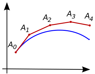
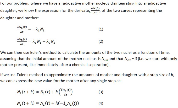
There is several different ways to numerically solve a differential equation. One of them, and the one we suggest you use here, is Euler's method. This method is based on that we know initial value of the function we are seeking a solution for - which for us is the initial amount of the daughter nuclei - and that we have an expression for the derivative of this function. The derivative is of course our differential equation. Since the derivative is the slope of the unknown function we are seeking, we can estimate the value close to a known point (the initial point) by moving along the tangential line with the same slope. See the graphical illustrations to the right (copied from Wikipedia). The blue line is the unknown function, the red line is the stepwise approximation starting in A0.

The error in each step (the discrepancy between our approximated point and the true value) is going to increase the further away from the initial point we get. It is a first-order method, which means that the local error (error per step) is proportional to the square of the step size, and the overall error is proportional to the step size.

A good description of Euler's method can be found on Wikiepedia, please refer to this or to a course book in numberical methods for details.


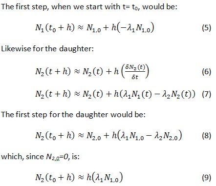
Use equation (4) and (7) to calculate the amount of mother and in-growth of daughter you will get for a selected time span. Make sure that the step-size you use is small enough to make the stepwise error negligible.

The Nuclear Chemistry Concepts you should Investigate

The numerical solution of the differential equation will enable you to plot the curves and illustrate the changes in desintegration rate of mother and daughter. In particular, you should look into the genetic scenarious suggested at the bottom of this page. Once you have code that enable you to calculate how much daughter you get as a function of time, you should use this to investigate graphically the genetic dependence of mother-daughter realtionships with respect of mother and daughter half-life scenarios.

From the analytical solution to the mathematical problem you can see how the half-lives of the two nuclei determine the genetic relationship. In particular you should notice and investigate how the fraction with the λs in front of A1 behaves for different combinations of mother and daughter half-lives. Likewise it is important to understand the role of the expression within the parenthesis - the "saturation factor". Work out the limit when t approches infinite!

As a concrete and also very important example, you should in particular investigate the 99Mo/99mTc-radionuclide generator. 99mTc is the most commonly used medical radionuclide in the world and the hospitals use generators with 99Mo attached to a column to produce the 99mTc.

We suggest that you write your program step by step and thoroghly check that each step works before you continue. You might want to follow the following path:

Step 1: Initialize parameters and get input parameters (amount and half-life of mother, half-life of daughter). You might also want to allow the user to specify the time interval to be modelled (keep careful track of the time units you use so you do not mix them up).

Step 2: Use both the analytically derived equation (approach A) and the numerical solution (approach B) to calculate the amount of mother and daughter (activity A1 and A2, respectivly) as a funcion of time. Store the results in two arrays 1000 elements long. You might find it convenient to also have a third array where you store the time for the respective elements in the two first arrays.

Step 3: Now you should plot your data. If you use a programing language that do not have good support for ploting, you might instead opt for generating a text file with the numbers to be plotted and import them into some appropriate plotting software. The plots should be semi-logaritmic (i.e. logaritmic scale along the y-axis, but not along the x-axis). Why do we want this? Your plots should have three different curves: 1) Sum of A1, A2, and background; 2) only A1; and 3) only A2. Both x- and y-axises should be appropriately labeled.

Step 4: Add functionallity to your program that allow you to either print or generate picture-files of your plots, as you will need to include them in your final report. If this is not possible with your choice of programming language you can do screen dumps, but this is never a good solution (nearly always too low-res).

Extras: Optionally you can select to also add a constant "background count rate", as a nuclear detector always will be exposed to this and therefore will be present and must be handled in a real measurement situation (you will most likely use the simulation program later when you do exercises that actually measure radioactivity).

Tips:

• The timestep for the numerical solution needs to be small enough for the method to be precise.

Investigate Genetic Scenarios

Now you can start using your program to learn more about radioactive decay! Investigate the following scenarios where you have a daughter nucleus genetically dependent on the mother:

• Short-lived mother, long-lived daughter (no equilibrium)
• Short-lived mother, short-lived daughter (no equilibrium)
• Relatively long-lived mother, short-lived daughter (transient equilibrium, T1/2(mother) >> T1/2(daughter)
• Very long-lived mother, short-lived daughter (seqular equilibrium, T1/2(mother > 104x T1/2(daughter))
• Examples of operation of a radionuclide generator, e.g. the 99Mo -> 99mTc generator. How much activity will you get after one, three and 10 daugher half-lives? What happens if you milk the generator two times in a row?