NucWik - Probability and Distribution

Back to Measurements uncertainty and Detection Limits

Probability in Radiation Counting

Consider a source with n radionuclides of a certain kind. According to the exponential decay model the probability of decay of a specific atom is 1-e-λt where λ = decay constant and t = counting time.
The probability of radiation emission, F (= the branching ratio I), is a characteristic of the radionuclide.
The probability of detection is the same as the counting efficiency ε.
Then, the probability that at an atom will generate a count in a certain detector within the time t is:

$p=\left( 1-e^{-\lambda t}\right) \cdot F\cdot\epsilon$

If the source with n radioactive atoms is counted on a detector with constant efficiency and its background is negligible, the number of observed counts S has a binominal distribution with parameters n and p.

The counting uncertainty of S is the standard deviation of the theoretical distribution of counts observed in a fixed time period when the efficiency is held constant.
Thus, the actual variability observed in repeated measurements of a single radioactive source may be greater than the theoretical counting uncertainty due to actual variation in counting efficiency etc.

Probability Distributions of Interest

Binomial Distribution

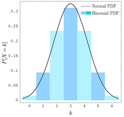
One may use the binomial distribution law to find the probability Pr(X=k) of obtaining just k disintegrations in time t from n original radioactive atoms.
If X is binomial with parameters n and p, then for 0 £ k £ n, the probability that X=k is given by the formula:

$Pr(X=k)=\frac{n!}{(n-k)!\cdot k!}p^k\cdot (1-p)^{n-k}$

Eqn. 1

The mean and variance of the binomial distribution are np and np(1-p), respectively. Normally, p is small enough for the factor (1-p) to be ignored.
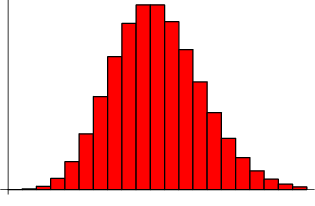
When this is true, the binomial distribution can be approximated by a Poisson distribution with the mean m = np.
The variance of a Poisson distribution equals the mean. Both can be estimated by the same measured result S, and the standard deviation can be estimated by s = (S)1/2.
If the mean is large, the distribution is well approximated by a normal (Gaussian) distribution.

Poisson Distribution

If X has a Poisson distribution with mean m, then for any non-negative integer k, the probability that X=k is given by:

$Pr(X=k)=\frac{e^{-\mu}\cdot \mu^k}{k!}$

Eqn. 2

Example of Combined Uncertainty

The content of 210Po (alpha emission) in water is measured by alpha spectrometry after the following sample preparation: A certain volume of water is contacted in an electroplating container where a nickel planchlet is mounted in the bottom. Polonium will quantitatively plate out on the planchlet by the mechanism of electroplating. The alpha decay rate per unit volume of the original sample solution is described by:

$D=\frac{\frac{S_s}{T_s}-\frac{S_b}{t_b}}{\epsilon\cdot V}$

Eqn. 3

where
SS=the accumulated counts for the source (SS=220)
SB=the accumulated counts for the background (SB= 55)
tS=the source counting time (tS=7200 s)
tB=the background counting time (tB=7200 s)
ε = the total counting efficiency (ε = 0.185)
V = the volume analysed (in contact with Ni) (V = 0.1000 L)
u(ε) = uncertainty in the counting efficiency (u(ε) = 0.010)
u(V) = uncertainty in analysed volume (u(V) = 0.0002 L)

Solution: First compute the output estimate for D from Eqn.3:

$D=\frac{\frac{220}{7200}-\frac{55}{7200}}{0.185\cdot 0.100}\approx 1.24\, dps/L$

Then compute the combined standard uncertainty from the uncertainty propagation formula,- explicitly:

$U_c^2(D)=\left(\frac{\delta D}{\delta S_s}\cdot u(S_s)\right)^2+\left(\frac{\delta D}{\delta S_B}\cdot u(S_B)\right)^2+\left(\frac{\delta D}{\delta S_\epsilon}\cdot u(S_\epsilon)\right)^2 + \left(\frac{\delta D}{\delta V}\cdot u(V)\right)$

Eqn. 4

The Poisson model is used to calculate the standard uncertainties of the counting numbers for the source and the background. This gives for the variance:

$u^2(S_s)=S_s=200 \, and \, u^2(S_B) = S_B = 55$

Partial derivation of Eqn.4 gives after inserting the relevant parameter values:
$\frac{\delta D}{\delta S_s}=\frac{1}{t_s\cdot\epsilon V}=0.0075075$

$\frac{\delta D}{\delta S_B}=\frac{-1}{t_B \epsilon V}=-0.0075075$

$\frac{\delta D}{\delta V}=-\frac{\frac{S_s}{T_s}-\frac{S_B}{t_B}}{\epsilon\cdot V^2}=-12.38739$

$\frac{\delta D}{\delta \epsilon}=-\frac{\frac{S_s}{T_s}-\frac{S_B}{t_B}}{\epsilon^2\cdot V}=-6.69588$

Inserting these values into Eqn.13 gives the combined variance:

$U_C^2 (D)=(0.0075075)^2\cdot 200+(-0.0075075)^2\cdot 55+ (-6.69588\cdot 0.010)^2+(-12.38739\cdot 0.0002)^2$

$u^2_c(D)=0.10445$

$u_v(D)=\sqrt{0.10445}\approx 0.32$

$\underline{D=1.23\pm0.32\, Bq/L}$